UPDATED ON AUGUST 4, 2021, the incorporation of extra-inning baserunners for the 2020 and 2021 seasons changed the original calculations, thereby improving the estimated runs predicted by pOR1 and pOR2.
Predicted Outcomes Runs is the most accurate and sophisticated publicly available runs formula/algorithm ever created.
The way in which I stumbled into the process of researching and eventually crafting the algorithm was covered in the general audience article available on this website. This column is intended for those who would like to understand POR’s details or see the corresponding statistical analysis. As such, this piece may get relatively thick with jargon. I would like to apologize upfront for any confusion you may experience. I will do my best to share representative examples where appropriate to increase understanding.
The first business to discuss is Predicted Outcomes Runs, or POR as I was calling it, has already undergone a massive revision. While I always anticipated the possibility of revising the formula if a real-world application proved insufficient to the task, I did not expect it to happen so soon. I’ll circle back to that in a moment—there’s my lone political jab, for those of you who may read my political or social articles on other sites—but before I do, I would like to point out my distaste for formulas that require constant revision.
I have always disliked formulas or algorithms for any discipline—baseball in particular—that need ongoing adjustments. Those formulas are not universally explanatory and unquestionably not predictive if they are not at least somewhat stable in their year-to-year turnover. Moreover, any formula that meets these criteria is only descriptive of the year it is applied. It has no universal appeal.
That level of accuracy may be sufficient in examining season-to-season baseball. It is wholly inadequate at describing what happened in any of the years before the formula’s specific weighted adjustment. It is equally unable to predict future years or likelihoods. To be succinct, it is a photograph in time—or a screenshot, to use the kids’ hip lingo. It doesn’t tell us anything that happened before or after the picture was taken as a single image. It would take 146 such photos to gain an understanding of the history of baseball. Still, there would be no possible image to predict what we might expect in years to come. Why not just craft a better metric that supplants the need for constant tinkering?
Now that you are aware of my aversion to non-universal universal formulas, I can proceed with explaining why I am already changing POR. To develop a unified theory describing all past, present, and future runs in professional baseball, I had to take a macroscopic approach to the analysis. Frankly, there was no other reasonable alternative when considering we are talking about 146 years of Major League Baseball. During that time, 230,000 games have been played, more than 2,000,000 runs have been scored, and approximately 60,000,000 pitches have been thrown. It is a massive data set, but more on that later.
With the formula constructed and tested over a handful of weeks, it was time to release it to the public. That hallmark came and went last week. I took the next day off to relax and then dove into a micro-level analysis of current data. Specifically, I began to apply my algorithm to individual box scores. I chose this to avoid a pitfall that befell one of my baseball idols—fellow Kansan, Bill James. In case you didn’t know, James’ Runs Created algorithm was criticized for its initial lack of success in explaining small sample sizes. With the benefit of hindsight, I hoped to get a jump on not falling victim to the same dilemma.
After several days of examining box scores to run them through the algorithmic calculator, I saw two trends in the micro-data that warranted immediate investigation. The first trend was the percentage at which home runs represented a team’s total bases for a particular game. Here is a chart that describes the trend:
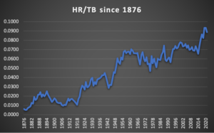
It’s not all that surprising if you watch baseball regularly. Still, putting actual numbers to the trend means that understanding the value of the home run as a percentage of total bases and any hidden runs scored is critical to developing any unified runs theory.
The second trend wasn’t as stark, though it’s had more of a universal impact on the game. Specifically, I’m referring to double plays. Initially, I chose to examine batters grounding into double plays. This is a data point used by most of the other significant runs estimation formulas. It seemed like a good place for me to start, too—shame on me for not following the data from the get-go on that.
You see, baseball has a double play gap—a big one. Roughly 90,000 double plays over the history of baseball are not the result of a batter grounding into a double play. Failing to account for this meant I was either missing an impactful event or overvaluing the impact of GIDP because I mistakenly thought it more closely matched the total number of double plays. For the record, flubbing on that many double plays translates into missing about 70,000 runs, or just less than one run every three games.
As a result of my discovery, I abruptly stopped the micro-analysis and jumped back into the formula for further development. What I found astonished me. Including all double plays meant adjusting the internal weight of numerous variables. When this process was complete, the final results were beyond what I could have hoped for. As a teaser, the second (and final, unless some third party discovers something I just can’t see) generation of POR—pOR2–has an accuracy rate I didn’t think possible without outside help from the sabermetric community.
The standard deviation for the entire data set when using pOR2 is under two percent. The actual value is 1.852% – 1.868%, depending on whether we accept the face value of percentage stats like BAbip, OBP, OPS, and SLG, or calculate the data based on the formulas that produce those percentages. The closest competitor to pOR2 is POR, or pOR1, as I am now calling it. The other runs estimators—remember, I don’t give annually-weighted algorithms any standing in this arena—are being lapped in terms of overall accuracy.
Okay. That was a lot to cover, and I still haven’t touched on the details of the formula. I felt it was vital for you to know the backstory of pOR2’s development to appreciate its value. Having said that, I want to reiterate the size of the data set I examined.
Constructing a gargantuan data set meant pulling information from multiple sources. Most of the season-by-season data came from Baseball-Reference. They are the only site I am aware of that houses that level of detail for the entire history of baseball unless you go with a paid subscription to one of the bureaus. Other sources, including this website—Baseball Almanac, were FanGraphs, Retrosheet, and Team Rankings. I cross-referenced some of the more unstable data points with bureau data before deciding what to include or ignore. I also elected to include Negro Leagues Professional Baseball data—where it exists—as they have thankfully been recognized as major leagues. I cannot overstate this point because it is foolhardy to ignore how the game was played by countless professionals who were just as good as their contemporaries in whites-only leagues yet denied the opportunity to participate. I will not entertain any historical review that does not include NLPB data.
Once I had the hulk of the data set in place, I had to check it for errors. This was a more cumbersome task than you might expect. Even within the Baseball-Reference library, the batting, pitching, and fielding totals don’t always agree. What is counted in one category doesn’t always appear in the corresponding category under the other umbrellas. The most salient example of this is with stolen bases and caught stealing. The fielding warehouse data include SB and CS data that don’t correspond with the batting warehouse. (The CS gap between the two is around 61,000, while the SB gap is approximately 4,000). As a result, I chose to use the fielding totals for these categories because they were more complete. Another reason to include examples such as this is that I knew I would have to build an inferential sample within the data set for missing information. Now, before you bristle at that, please read on to learn how I went about it.
To build the inferential (best logical guess) data sample, I had to set aside the data set until I mapped the historical trends of relevant events within the games and the outcomes of those games. My findings deserve their own column (or several) and will be the subject of a future article. If I may share a few highlights with you, several event outcomes that occur within the games themselves have been remarkably stable over the game’s history. These include batting-average-on-balls-in-play (BAbip), hit by pitches, and walks. Even home runs, with their relative spike in frequency, have remained relatively stable. The only constant event that has been with us throughout the history of baseball that has seen a dramatic shift is the strikeout.
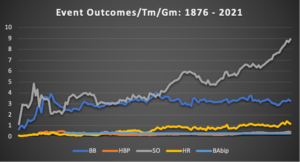
You can see the trend-lines in the chart above. This representation is intended only to offer a barometer of how the game has been played. Of course, there have been many changes to strategy over the years. Books, radio and television shows and other media types devote countless hours to dissecting the nuanced differences between different “eras” within baseball. Again, that’s a story for another day. Despite many changes in event outcomes within the games that may have actually occurred or been perceived to have altered the game in some dramatic fashion, those shifting event outcomes didn’t impact the observable game outcomes.
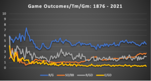
Here again, we can see a trend-line chart illustrating numerous game outcomes since 1876. Following some early chaos in the data from 1876 to 1900, the game abruptly stabilized at the league-outcome level. Runs-per-game-per-team has never fallen below three runs, nor has it risen above six since that time. The same is true for the differential between the league’s highest and lowest scoring teams. This gap, referred to as a game-differential, tells us that despite any changes in event outcomes within games, the outcomes of the games remain the same—teams score roughly the same amount of runs per game as they always have, and the gap between the highest and lowest scoring teams in the league is where we would expect it to be.
The other differential I wanted to investigate was in errors per game. A similar result occurred wherein the chaos of early baseball gave way to a stable atmosphere that tells us a good deal about the importance of defense in the game. Errors have virtually disappeared from baseball, as evidenced by the gap between the team that committed the most errors and the team that committed the fewest errors.
I need to tell you that I had to make another executive decision about which teams to include in these results. Since I included NLPB teams in my study, when examining runs-per-game-differential (R/GD) and errors-per-game-differential (E/GD), I could only include those NLPB teams that played a minimum of 80% of the total number of games played by the MLB team that played the most games in a particular season. It would have been statistically invalidating to include teams that played significantly fewer games.
The salient highlight to share with you here is that the E/GD between the “best” and “worst” defensive teams has all but vanished. Since 1954, the gap in errors-per-game has remained stable at 0.4 errors. In layman’s terms, it means the “worst” defensive team each season commits one more error every 2.5 games than the best defensive team. Over a 162-game season, this is about 65 errors, or about 23 more runs allowed defensively than the best defensive team. That is about 1/7th of a run each game because of “bad” defense.
Alright. I hope you’re still with me. If you’re wondering why I devoted so much time to the historical trends, there is a valid reason. These trends were necessary to provide the underlying premises of any data modeling I chose to attempt. They illustrate something referred to as the law of large numbers. Essentially, this is a theory within statistics that tells us that the more an experiment is conducted, the greater the likelihood the results will mirror the average member of the population. Thinking back on the size of the data under investigation—230,000 games, 15,000,000 at-bats, etc.—each event, whether one more minor event within a specific game or an outcome of the game itself, is now two data points because it includes an offensive player and a defensive player. Ultimately, it means we have tens of millions of data points between mutual combatants (batters versus pitchers, runners versus fielders) with which to draw statistically reliable conclusions and make universal declarations.
The historical review informed me of more than just which data to include and exclude in my data set. I was also able to determine a breakpoint for historical averages that mirrors actual breakpoints within the historical data itself. The cleanest breakpoint for determining historical averages is between the years 1900 and 1901. If the period from 1876 – 1900 (I refer to this era as the formative years of baseball) is temporarily removed from the data set to identify trends, the historical per-team-per-game averages from 1901 to the present look surprisingly similar to a modern box score. Teams averaged a .299 BAbip (or .2847, if we calculate BAbip using the data available and the corresponding formula), scored 4.42 runs per game with an R/GD of 1.92, and an E/GD of 0.54. The obvious conclusion is that historical averages from 1901 to the present can be applied as universal averages to the data set and any predictive modeling it provides.
With the historical analysis complete, I returned to the data set to find which variables belonged in a unified formula and which did not. To accomplish this, I wanted to identify the historical correlation between each in-game event outcome and runs scored. I calculated an 1876 – 2021 correlation and a 1901 – 2021 correlation. The purpose of using two correlations of event outcomes was to observe any discrepancy between the two to identify how the game was played before 1901 when baseball was still undergoing spasmodic changes as it was being codified. It should come as no surprise that RBIs, TBs, 1Bs, and 2Bs are the statistical events most closely related to scoring runs. I encourage you to take some time to review the accompanying data to see for yourself. What was interesting was to discover which events bore little relationship to scoring runs.
Before I discuss the correlations, I want to make a quick point about correlation and causation. Anyone who has taken a statistics class will tell you that correlation does not equal causation. Well, duh. That doesn’t remove or diminish the value that correlated events have. Even non-causative correlations are extremely telling. I used a non-causative analysis to eliminate factors in my box score micro-analysis to identify which events I had overlooked. The bottom line is correlation matters.
After identifying which raw statistical events I would include in my formula, I discovered that I needed to actually devise or record first-level analysis statistics to explain the phenomena I observed. Perhaps the statistics I created already exist. Still, they are not stored as universal data on any publicly available platform, which meant I needed to record them for my own use. These statistics include Bases taken plus errors (BtE), Awarded first base (A1b), and All bases gained (Abg). Each of these stats has two derivatives divided by the number of total bases or plate appearances. I also created similar derivatives for caught stealing plus pickoffs divided by TB or PA, home runs per TB, walks per TB, and runs per TB. Having said that, not every new statistic or its derivative made it into the final formula; yet, each helped me to see the game in a slightly different way than raw data permits.
The formula itself is a bit of a mad scientist’s creation. It is large, unwieldy, and generally ugly. At the same time, its characteristics are beautiful to me in their simplicity. Specifically, I have eliminated any need for weighted averages for the formula and algorithm by designing a way to build those weights into the formula’s internal calculations. It means a person can simply input the raw data and receive the predicted runs total and see how the formula calculates percentages that will reflect player, team, or league percentages relative to their average in a given year. This is captured by using the percentages—OPS, OBP, and BAbip—as the global multipliers on the top and bottom halves of the formula. The formula uses thirty-one separate variables to calculate runs over forty-two different calculations. Some variables appear more than once in the formula, be it in the top or bottom halves.
Here is the formula, which I will explain below:
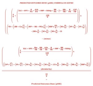
As discussed, the formula has top and bottom halves. Think of these like the buttons on an analog radio or the dials on a telescope. The top half of the formula is the dial, and the bottom half tunes the result. Through this series of operations, specific variables can be included twice as both a gross total in the top half and a tuning adjustment for detail in the bottom half. This also means that specific statistics are “tuned” in the bottom half while not appearing in the top half. If this seems confusing, it implies that those particular data points are relevant to run-scoring but not in need of the gross adjustment that comes from being included in the top half of the formula. It should also be noted that three additional variables which do not appear directly in the formula are used purely for calculations. These are hits (H), plate appearances (PA), and at-bats (AB). Without these additional elements, the percentage-based “dials” could not be “tuned.”
As with the first generation of pOR, pOR2 uses multiples of sixths to assign the correct value to each corresponding calculated event. I mentioned this briefly in the general audience article. The presumption behind this was that baseball games are themselves divided into sixths. I highlighted the innings of a baseball game as the “nine sets of sixths” in that column. However, there is a further subdivision if you remember that within each data point, there are two entries: one for the offense and another for the defense. This tells us that each pitch, ball in play, hit, or out is two data points. Ultimately, for the formula, it means that each out needs to be multiplied by two to reflect its value for both combatants (batter versus pitcher, runner versus fielder). Anything less would severely limit the ability to tune the formula.
Something else you may be wondering is why the need for so many variables for the formula. My answer is the same as what my father said to me many times: do you want speed or do you want accuracy?
In the instance of explaining where all runs in professional baseball come from, accuracy trumps speed. Frankly, we’ve seen what the other runs estimation algorithms do with less and “less” is not sufficient for the task. Furthermore, I set aside my ego when inputting various combinations. It simply didn’t matter what it took to get the formula and its corresponding algorithm correct. What mattered was getting a product that is miles better in every measurable way. To that end, it’s time to share the main attraction: the statistical analysis.
pOR2 is the eighth generation of the formula I constructed to adequately describe, measure, and predict runs scored in professional baseball. pOR1 was the fifth version, though the first to go live. Until the advent of pOR2, pOR1 was the most accurate runs algorithm ever created for public use. I’ve already shared the standard deviation for the overall population (1.852%). Where pOR2 shines is in its subpopulation results.
| 1876 Correl | 0.9988 | 99.855% | Season/E | |||
| Year | Tms | G | R | pOR2 | StDev | R/Tm/GE |
| Totals since 1876 | 0.9988 | 1.868% | 0.0066 | |||
| The Formative Years | 0.9990 | 2.814% | 0.0469 | |||
| The AL, NL, and NLPB | 0.9959 | 1.792% | 0.0361 | |||
| Major League Expansion | 0.9988 | 1.091% | 0.0181 | |||
| Post-Expansion MLB | 0.9971 | 1.992% | 0.0115 | |||
| 1901 Correl | 0.9985 | 1.620% | 0.0028 | |||
We have the 1876 – 2021 correlation of 0.9988 and the percentage of runs the algorithm predicted for the entire set in the top row. You will notice it says 99.855% and not the advertised 99.988%. The reason for this is I decided to play around with the data set once again, this time correcting the values of stats like BAbip, OBP, OPS, and SLG to their values based on the presented data rather than taking the face value of the original stat as presented by Baseball-Reference. I am not suggesting BR is or is not correct in their interpretation. I wanted to show the statistical results as calculated by their respective formulas on one worksheet (above chart) and another using the statistics at face value from BR.
Returning to this chart, the subpopulations were 1876 – 1900, referred to as The Formative Years; 1901 – 1953, The AL, NL, and NLPB; 1954 – 1997, Major League Expansion; and 1998 – 2021, Post Expansion MLB. I have also noted the period from 1901 to the present in the bottom row of this chart as the 1901 correlation. So, for the entire population, there is a 99.88% relationship between runs scored and pOR2; a 99.90% relationship for the Formative Years, a 99.55% relationship for the AL, NL, and NLPB years; 99.88% relationship for the Expansion years; and a 99.70% relationship for the Post Expansion years. We can also see the correlation since 1901 shows a 99.85% relationship between pOR2 and runs scored for the last 120 years combined. Simply put, these are exceptionally high numbers. By comparison, of the competitors tested, Runs Created Technical (by Bill James) comes closest to the 1901 correlation at 99.64%. The truth is even to get close to the levels described by pOR, I had to create a two-standard-deviation model that excluded all years from the calculation if they fell outside of two standard deviations (margins of error) of my results. Put another way, I simply canceled out the years from the calculation if they were more than 3.704% away from the 99.988% runs predicted by my algorithm. Only when I did that did a single competitor exceed my metric (Jim Furtado’s Extrapolated Runs). However, it should be noted that even in this instance, XR could only accurately predict 77 of 146 years while pOR2 still predicted 140 of 146 years, though XR did so with a higher degree of reliability. Stating this yet another way means that Furtado could predict 62% of all runs with near-certain accuracy (correlation of 0.9993) while I predicted more than 97% of all runs with almost the same accuracy (correlation of 0.9991).
Setting aside the unusual models that had to be created to demonstrate the ability of my competitors, all algorithms were subjected to the same data set for the battery of tests. Available data for all observed categories exists back to 1954. Before that year, data collection for each statistical category is hit and miss (Get it? Hit and miss! Ah, dad jokes). In some cases, the statistical measure in question didn’t exist as a separate measure, as in the case of the sacrifice fly (SF).
To overcome these dilemmas, a random array sample was created based on 1-year, 3-year, and 5-year averages to provide a universal set that could include all relevant data for all years of the study. If those averages trended in the opposite direction of the historical trends, a combination of trend and average data was used to create the random array set. After the array’s limits were compiled, I had Microsoft Excel generate random percentages for measures like stolen bases or caught stealing for the years where data did not exist. The parameters of the array meant the software would not generate results outside of the accepted boundaries.
To test the algorithms side-by-side, each was expected to perform with the margin of error set forth by pOR2. This means each algorithm needed to accurately predict 98.136% – 101.840% of runs for a given year. Since each algorithm was subjected to the same random array sample, reasonable conclusions can be drawn regarding the reliability each algorithm possesses to describe or estimate runs from 1876 to 1953. The competing runs estimators that were tested are David Smyth’s Base Runs Raw (BsR), Paul Johnson’s Estimated Runs Produced (ERP), Jim Furtado’s Extrapolated Runs (XR), and Bill James’s Runs Created Technical (RCt). Unfortunately, none could estimate the period from 1876 – 1953 with any degree of accuracy or reliability.
For the 78 years from 1876 – 1953, BsR predicted two years within the margin of error. ERP estimated zero years within the margin of error; RCt estimated four years within the margin of error; and XR estimated three years within the margin of error. By comparison, pOR1 estimated 54 years within the margin of error, while pOR2 estimated 49 years within the margin of error. This is one of the few instances where pOR1 outperformed pOR2.
When the same period (1876 – 1953) was adjusted to include two margins of error, the results did not improve for the competitors. BsR could only estimate eight years with an accuracy of 96.284% – 103.692%. ERP estimated five years within this broader margin; RCt estimated 17 years accurately; and XR estimated nine years accurately. Again, by comparison, pOR1 estimated 70 years accurately, while pOR2 estimated 73 years accurately.
Overall, these underwhelming results persisted when the study period included all 146 years of major league baseball. BsR accurately estimated 52 years within one margin of error; ERP estimated 51 years accurately; RCt estimated 49 years accurately; and XR estimated 59 years accurately. pOR1 estimated 109 years accurately within one margin of error, and pOR2 estimated 107 years accurately. If accuracy were broadened to two margins of error, pOR1 accurately estimates 137 years, while pOR2 accurately estimates 140 years. By any measure of estimation or prediction, the competing runs estimators are barely half as accurate as pOR.
Another measure of reliability is how many of the 2,088,087 total runs scored each algorithm estimated. BsR, RCT, and XR each estimated just over 95% of the total runs scored, while ERP estimated just under 95% of total runs. pOR1 and pOR2 each estimated over 99.97% of all runs scored. Even if we examine only the period from 1901 to the present, none of the other metrics could estimate 99% of the runs scored, while both pOR formulas predicted 100% of total runs. The bottom line is that the only runs estimator competitive with pOR2 is pOR1.
You may be wondering why I keep comparing the two released generations of pOR. I want to highlight the strength of each while showing the exceptional lengths that pOR2 goes to in explaining historical runs and predicting future runs. One way to determine this is to look at the regression analysis for each algorithm.
| pOR1 | pOR2 | ||
| Multiple R | 0.9987 | Multiple R | 0.9988 |
| R Square | 0.9974 | R Square | 0.9976 |
| Adjusted R Sq. | 0.9974 | Adjusted R Sq. | 0.9976 |
| Standard Error | 261.88 | Standard Error | 252.27 |
| RMSE | 260.08 | RMSE | 250.54 |
| Sum of Squares | 99.74% | Sum of Squares | 99.76% |
| P-value | 1.82e-188 | P-value | 8.38e-191 |
As you can see, the regression analysis statistics are extraordinary. The MR, RS, and ARS values define the strength of the relationship between each algorithm and runs scored. The SE and RMSE estimate the error within the model’s design. The SS tells us how much variance, or overall data points, are accurately predicted by each model. Finally, the PV tells us the likelihood that each model was arrived at by chance. For the sake of comparison, none of the other tested runs estimators came close in any of these categories.
I want to repeat something I said in the general audience article. I have nothing but great respect and appreciation for the other people who have created runs estimation formulas and algorithms. Without their work, I wouldn’t have been able to do this. At the same time, with the power of modern computers, it was time to conduct a better test under stricter conditions that used actual correlated measures to identify where runs come from.
We’ve come to the part of this report where I admittedly grimace. Before I describe the “run shares” that each of the raw statistical measures contributes to a run, I need to explain that these are only averages over millions of data points. They do not and cannot represent specific games to produce reliable results in a single example. Their reliability and accuracy come from repeated tests over many games. Nevertheless, I suppose it’s time to describe the run share that each batting or baserunning event contributes to run production.
| Run shares by event: | ||||
| 1 TB = 0.44 runs | 2.27 TBs = 1 run | 1 HBP = 1.41 runs | 0.71 HBP = 1 run | |
| 1 BB = 0.47 runs | 2.13 BBs = 1 run | 1 Pick-off = -0.03 runs | 40 POs = -1 run | |
| 1 DP = -0.79 runs | 1.27 DPs = -1 run | 1 SB = 0.58 runs | 1.72 SBs = 1 run | |
| 1 SF = -0.50 runs | 2 SFs = -1 run | 1 SH = -0.25 runs | 4 SHs = -1 run | |
| 1 HR = 2.34 runs | 0.43 HRs = 1 run | 1 CS = -0.45 runs | 2.22 CSs = -1 run | |
| 1 WP, BK, or PB = 0.007 runs | 14.29 WP, BK, or PBs = 1 run | 1 E = 0.36 runs | 2.78 Es = 1 run | |
| 1 SO = -0.16 runs | 6.25 Ks = -1 run | 1 “other” out = -0.07 runs | 14.29 “other” outs = -1 run | |
It may seem counterintuitive that certain events associated with run-scoring events would have a negative run-share-value. This is a product of the cost of the associated “out” attached to those events. Specifically, sacrifice flies are the prime example. Yes, a run is scored on a SF. An out also accompanies that event. For reasons I can’t explain because I don’t understand them completely, these events only produced “value” for the algorithm when they were assigned a negative value in the formula. All of this leads into the final piece I want to discuss in this column.
As I said in the general audience piece, I want this algorithm to be a tool for others as it is for me. If more imaginative minds than I can improve upon it, I am happy to support them in their efforts with what I can. I don’t believe that pOR is perfect. I don’t believe in a “perfect” metric. I think each generation of statistical measures moves us one step closer to providing ever more detail to the map of baseball. Thanks for staying with me along this long and windy road. I’m happy to answer any questions you may have.
Excel Workbook:
pOR2- Algorithm Comparisons – BsR, ERP, pOR1, RCt, and XR
Excel Baseball Outcomes Calculators: